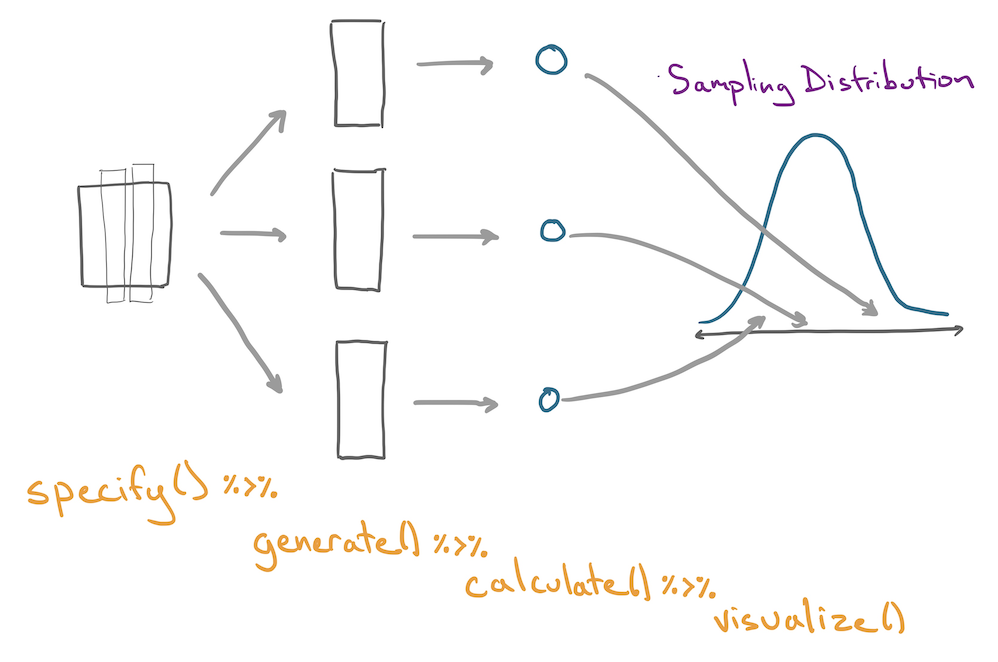
This tutorial utilizes several functions from the infer library, which can be used to calculate confidence intervals via the bootstrap and conduct hypothesis tests via a few different methods. It can be loaded with library(infer).
The specify function allows you to specify which column of a data frame you are using as your response variable (your variable of interest). When looking at the relationship between two variables you will specify both the response and the explanatory variables. As such, the main arguments are response and explanatory.
Observe that the output of specify is essentially the same data frame that went in. the only difference is that bill_length_mm is tagged as the response variable. That will be useful for downstream functions.
Working with categorical response variables
bill_length_mm is numerical. Say you’re working with a categorical variable and want to estimate a proportion. Since there are usually at least two levels (options) in a categorical variable, the specify() function will ask you: “the proportion of what level?” You need to tell specify() which level explicitly. This can be done with the additional success argument! Below, we are telling infer that we are interested in estimating the proportion of all Antarctic penguins that are female. Make sure the column name is in quotes.
Response: sex (factor)
# A tibble: 333 × 1
   sex
   <fct>
 1 male
 2 female
 3 female
 4 female
 5 male
 6 female
 7 male
 8 female
 9 male
10 male
# ℹ 323 more rows
The generate function generates many replicate data frames using simulation, the bootstrap procedure, or shuffling. Note that it must follow specify() so that it knows which column(s) to use.
Useful functions include:
reps: the number of data set replicates to generate. Generally set this to 500 when making confidence intervals.
type: the mechanism used to generate new data. Either "bootstrap", "draw", or "permute". Today, we’ll be using the bootstrap; the other two argument choices will be explained in subsequent lectures!
penguins |>specify(response = bill_length_mm) |>generate(reps =2, type ="bootstrap")
the output data frame has two columns, replicate, which keeps track of the replicate (1 or 2 here) and bill_length_mm.
the number of rows in the resulting data frame is the \(n \times reps\), so this data frame is contains all of the bootstrap replicate stapled together one on top of another.
The third link in an infer pipeline is the calculate function, which calculates a single summary statistic for each replicate data frame. The main argument is stat, which can take values "mean", "median", "prop" (for proportion), "diff in means", "diff in props" and a few more.
penguins |>specify(response = bill_length_mm) |>generate(reps =2, type ="bootstrap") |>calculate(stat ="mean")
Response: bill_length_mm (numeric)
# A tibble: 2 × 2
  replicate  stat
      <int> <dbl>
1         1  45.1
2         2  43.9
Observe:
The name of the summary statistic should be put in quotation marks.
The resulting data frame had reps rows, one statistic from every replicate.
The calculate function is a shortcut for an operation you’re familiar with:
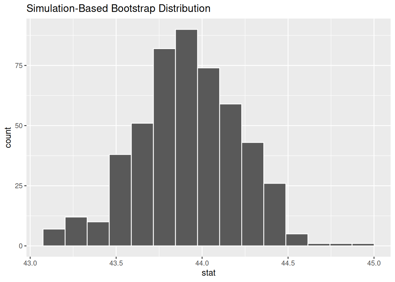
Now imagine that we have a distribution of many bootstrapped statistics (a bootstrap sampling distribution). Let’s put that distribution on a histogram! Normally, we’d have to use ggplot() to do this, but the infer library offers a nifty function called visualize() which does this for us in one easy step (and even titles the plot appropriately!) Here, we’ll plot a sampling distribution of 500 bootstrapped means.
The moment we’ve been waiting for is here– it’s time to calculate the confidence interval! For a 95 percent confidence interval, we’ll leave out 5 percent of the sampling distribution: 2.5 percent on the low side, counting up from 0 percent, and 2.5 percent on the high side, counting down from 100 percent. Therefore, we’ll take the 2.5th percentile and the 97.5th percentile of our distribution as the lower and upper bound, respectively.
Luckily, the get_ci() function does this work for us! Its level argument allows us to specify the confidence level we’d like.
If you would like to create bootstrapped coefficients for a linear model, you’ll have to do something a bit different since there is a more than 1 summary statistic involved for each replicate data set. This is the role of fit(). There are no arguments to fill-in; it inherits the formula for the linear model from specify().
penguins_adelie <- penguins |>filter(species =="Adelie")penguins_adelie |>specify(body_mass_g ~ sex + flipper_length_mm) |>generate(reps =2, type ="bootstrap") |>fit()