Continuous Distributions and Normal Approximations
Connections to boxes, continuous distributions, and a fundamental result
Ideas in code
Useful functions
Uniform\((a, b)\)
dunifcomputes the density \(f(x)\) of \(X\) where \(f(x) = \displaystyle \frac{1}{b-a}\), for \(a < x < b\).
- Arguments:
x: the value of \(x\) in \(f(x)\)min: the parameter \(a\), the lower end point of the interval for \(X\). The default value ismin = 0max: the parameter \(b\), the upper end point of the interval for \(X\). The default value ismax = 1
punifcomputes the cdf \(F(x) = P(X \le x)\) of \(X\).
- Arguments:
q: the value of \(x\) in \(F(x)\)min: the parameter \(a\), the lower end point of the interval for \(X\). The default value ismin = 0max: the parameter \(b\), the upper end point of the interval for \(X\). The default value ismax = 1
runifgenerates random numbers from the \(Unif(a,b)\) distribution.
- Arguments:
n: the size of the sample we wantmin: the parameter \(a\), the lower end point of the interval for \(X\). The default value ismin = 0max: the parameter \(b\), the upper end point of the interval for \(X\). The default value ismax = 1
Normal\((\mu, \sigma^2)\)
dnormcomputes the density \(f(x)\) of \(X \sim N(\mu,\sigma^2)\)
- Arguments:
x: the value of \(x\) in \(f(x)\)mean: the parameter \(\mu\), the mean of the distribution. The default value ismean = 0sd: the parameter \(\sigma\), the sd of the distribution. The default value issd = 1
pnormcomputes the cdf \(F(x) = P(X \le x)\) of \(X\).
- Arguments:
q: the value of \(x\) in \(F(x)\)mean: the parameter \(\mu\), the mean of the distribution. The default value ismean = 0sd: the parameter \(\sigma\), the sd of the distribution. The default value issd = 1
rnormgenerates random numbers from the Normal\((\mu, \sigma^2)\) distribution.
- Arguments:
n: the size of the sample we wantmean: the parameter \(\mu\), the mean of the distribution. The default value ismean = 0sd: the parameter \(\sigma\), the sd of the distribution. The default value issd = 1
Example
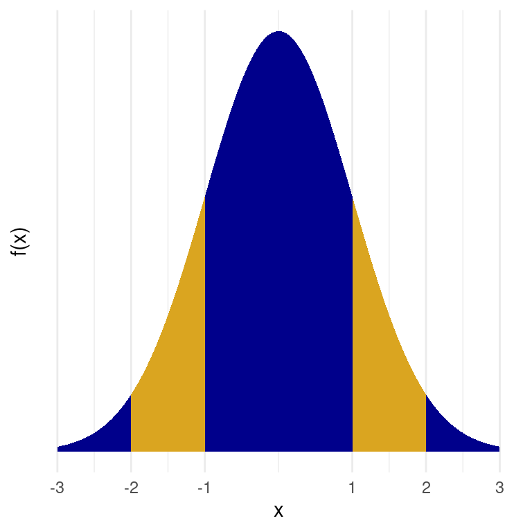
Let’s verify the empirical rule for the standard normal random variable:
Note that (for example) \(P(-1 \le X \le 1) = F(1) - F(-1)\):
pnorm(q = 1) - pnorm(q = -1)[1] 0.6826895pnorm(q = 2) - pnorm(q = -2)[1] 0.9544997pnorm(q = 3) - pnorm(q = -3)[1] 0.9973002The argument prob in the function sample()
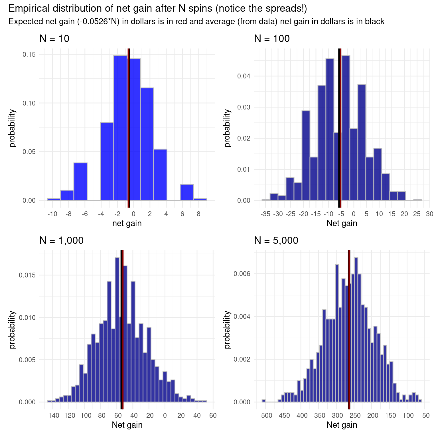
We have seen the function sample(), but so far, have only used it when we were sampling uniformly at random. That is, all the values are equally likely. We can sample according to a weighted probability, though, by putting in a vector of probabilities. Let’s look at the example of net gain while betting on red on a roulette spin. Recall that if we bet a dollar on red, then our net gain is \(+1\) with a probability of \(\displaystyle \frac{18}{38}\) and \(-1\) with a probability of \(\displaystyle \frac{20}{38}\).
gain <- c(1,-1) # define the gain for a single spin
prob_gain <- c(18/38,20/38) #define the corresponding probabilities
exp_gain <- sum(gain*prob_gain)
exp_gain
[1] -0.05263158set.seed(123)
#simulate gain from 10 spins of the wheel
sample(x = gain, size = 10, prob = prob_gain, replace = TRUE) [1] -1 1 -1 1 1 -1 1 1 1 -1#simulate net gain from 10 spins of the wheel which would sum these
sum(sample(x = gain, size = 10, prob = prob_gain, replace = TRUE))[1] 0Here is a simulation showing the Central Limit Theorem at work, with the empirical distribution becoming gradually more bell-shaped. Net gain is the sum of \(n\) draws with replacement from the vector gain defined above using the prob_gain vector.