| student_id | age | income_silver_marks | political_affiliation | city | height_feet |
|---|---|---|---|---|---|
| 1 | 30 | 45 | Guelph | Genoa | 5.78 |
| 2 | 21 | 28 | Guelph | Paris | 6.01 |
| 3 | 24 | 32 | Guelph | Siena | 5.81 |
| 4 | 21 | 16 | Guelph | Siena | 5.67 |
| 5 | 20 | 104 | Ghibelline | Verona | 5.77 |
| 6 | 24 | 39 | Guelph | Genoa | 5.79 |
| 7 | 23 | 30 | Guelph | Pisa | 5.53 |
| 8 | 28 | 34 | Guelph | Pisa | 5.88 |
| 9 | 18 | 32 | Ghibelline | Genoa | 6.02 |
| 10 | 22 | 79 | Ghibelline | Genoa | 5.95 |
Intro to Prediction
What is prediction and Ordinary Least Squares
WarningAfter reading, you should be able to explain the following…
- What prediction is.
- Leveraging generalization to make predictions.
- Target variable.
- Perfect generalization still leads to imperfect predictions.
- Leveraging association to improve predictions.
- Feature variables.
- Predictive algorithm.
- Baseline regression.
- Population mean squared prediction error.
- Linear regression.
- Residuals.
- Sample mean squared prediction error.
- Ordinary Least Squares regression.
- Iterative numerical algorithms.
Why did we do generalization to begin with?
In the generalization unit we did 2 things:
- Assume that the sample (the data, \(Y_1, Y_2, \ldots Y_n\)) came from a larger unknowable pattern or population (the distribution of \(Y\))
- Use the sample to guess something about the distribution of \(Y\) (e.g. estimate the mean \(\mu = E(Y)\) of the population using the mean of the sample: \(\bar{Y}\))
(Notice that I sneakily chose to use \(Y\) instead of \(X\) for the variable of interest…)
But why?
Well, sometimes we might just care about that specific number \(\mu\), for whatever reason, but, in a large number of cases, we have an implicit goal in the back of our minds: using that number to predict future data behavior!

E.g. Making friends on campus.
The year is 1247. Like always, university is about power and making connections. You’re a student from a modest family, and want to make friends with… well, rich students. There is bloody, fierce political divide on campus, though, and you want to be careful. Two parties, the Guelphs and the Ghibellines, are at each others’ throats.
A student, in his brown gown, walks down the path from the chapel and crosses your path. Do you want to approach him?
Luckily, you got data!
They ran a sampled survey a few years ago and recorded age, income (in silver marks), political affiliation, city of origin, and their height (in feet).
You could use this data to just estimate the population parameters, like means, proportions…
| num_students | proportion_Guelphs | mean_income_silver_marks |
|---|---|---|
| 120 | 0.5666667 | 30.65 |
But… you could also use that to make a prediction about the man walking up to you!
Given what you know about the data, would you guess the student is a Guelph?
You’ll probably say yes, but…
… you’ll feel a bit uneasy with this for several reasons.
- How do we know the data is indicative of the general pattern through the population?
- Is it morally OK to make guesses about people based on general patterns in the population?
- What’s the chance that my guess is just wrong?
How do we know the data is indicative of the general pattern through the population?
This is just the old problem of the generalization unit. Estimates from data are affected by uncertainty/error (bias, variance …). Nothing to add here. Making predictions from data is affected by this same issue. We inherit this original sin.
Is it morally ok to make guesses about people based on general patterns in the population?
This is tough. This is an ethical questions, an important one. Data problems, scientific problems are fraught with important ethical questions. We are not going to tackle it now, but it’s something that you absolutely must concern yourself with very soon in your life, if you’re going to act responsibly as a member of society. For the remainder of these lectures, we are going to make the working assumption that such ethical conundrums do not apply.
What’s the chance that I’m wrong about it?
Okay, this is where I wanted to focus your attention, to be honest. Even with perfect knowledge of the population, even with an infinite sample size, we would have a gigantic error rate of \(\approx 43.3\%\). Imagine if that was the rate at which a self-driving car makes a wrong turn. Completely unacceptable.
This suggests two things:
- We need to create a framework to measure the goodness of our predictions.
- We sure need to make more accurate predictions. But how?
Types of prediction
In making predictions, the most important question is “what do you want to predict?” The answer to that question is called the target variable (or response variable, or outcome variable, or dependent variable, or label, or other commonly used phrases, sigh…).
def: Target Variable
The random variable that is being predicted. Usually indicated by \(Y\).
Using the example above, the target variable would be \(Y =\) “Is this person a Guelph?”. “Yes” or “No”. A categorical binary variable.
In this case we talk about a classification task.
def: Classification Task
A task where we try to predict a categorical target variable.
In practice this definition works smoothly for nominal categorical variables. With ordinal ones… it’s a gray area, sometimes they might be turned into numerical variables instead.
Imagine trying to guess \(Y=\) the student’s annual income. A numerical variable…
def: Regression Task
A task where we try to predict a numerical target variable.
How to improve predictions? Association is back!
You are terrified to talk to the student because you have a \(\approx 43.3\%\) chance of being wrong about how they feel about politics.
How do we improve your chances?
Well, maybe you can test the water, so to say? For example you can ask some other information about them, like “What city are you from?”
| city | num_students | proportion_Guelphs | mean_income_silver_marks |
|---|---|---|---|
| Bologna | 8 | 0.7500000 | 23.37500 |
| Florence | 6 | 0.6666667 | 28.83333 |
| Milan | 7 | 0.4285714 | 34.28571 |
| Siena | 11 | 0.8181818 | 25.90909 |
| Pisa | 11 | 0.8181818 | 23.45455 |
| Lucca | 8 | 1.0000000 | 29.37500 |
| Perugia | 7 | 0.4285714 | 29.42857 |
| Rome | 5 | 0.2000000 | 29.00000 |
| Venice | 9 | 0.0000000 | 35.55556 |
| Genoa | 11 | 0.4545455 | 30.54545 |
See? We computed the same summaries (proportions and averages) but now broken down by a different variable (city of origin).
If he tells you he’s from Rome, what’s your guess? And what’s your chance of being wrong now?
Now I’m gonna guess he’s a Ghibelline! and I estimate that I have only a 20% chance of being wrong!
City of origin and Political affiliation are strongly associated (categorical) variables. It’s low-risk and low-cost to know their city of origin (\(X\)). We can use that variable to make a better guess at their high-risk hidden target variable, political affiliation (\(Y\)).
def: Features
The variables (indicated by \(X_1, X_2, \ldots X_q \equiv \mathbf{X}\) etc.) that are known and available for us to make the prediction about the unknown target variable (\(Y\)). Also called the independent variables or the predictor variables.
An apology about notation
I am sorry. Unfortunately we’ll need to change our notation. In the past we only used \(X_4\) to mean the fourth draw from a certain distribution/population, the fourth element in our sample. However, now by that we might also mean the fourth recorded feature in our datasetet, e.g. \(X_1 =\) “Name”, \(X_2 =\) “Height”, \(X_3 =\) “Sex”, \(X_4 =\) “number of children”, etc…
We’ll use \(\mathbf{X}\) to mean the set of all the features \(X_1, X_2, \ldots X_q\), and \(X_j\) for one of those features.
def: Predictive Algorithm (model)
A statistical procedure learned on old data (sample) that uses multiple available variables (features, or explanatory variables) to predict the value of an unknown target variable. This prediction or predictor is denoted by
\[\hat{Y}(\mathbf{X}) \mbox{ or } \hat{Y}(X_1,X_2,\ldots , X_q) \mbox{ or just } \hat{Y}\]
This scary expression is just saying that your prediction depends on the \(X\) variables.
Notice the “hat” symbol. Again, it indicates that this quantity depends on the old sample \((X_{1,1}, \ldots, X_{q,1}, Y_1), (X_{1,2}, \ldots, X_{q,2}, Y_2), \ldots, (X_{1,n}, \ldots, X_{q,n}, Y_n)\) (Ouch, this looks ugly). It was learned or fitted on the old sample, and now, it’s trying to make a prediction about a new generic data point \((X_1, \ldots, X_q, Y)\).
This is often referred to as the “model”. This usage might generate confusion in the reader with the related but distinct concept of “(parametric) model”, i.e. the assumptions we make about the distribution of a random variable.
The past two decades have been a golden age for predictive algorithms, with hundreds of new types being invented that can address regression tasks or classifications tasks or often both. To take a deep dive into this diverse landscape, take a course in Statistical or Machine Learning. For the purpose of this course, we’ll just take a dip and focus on two algorithms: Least Squares Linear Model for Regression and a Logistic Regression for Classification.
Regression: let’s talk numerical variables.
The baseline: The most boring regression algorithm you’ll ever see
What would you predict as the annual income of the student approaching you?
This is a regression task.
Go check the first summary table a few paragraphs above…
Yeah the sample mean for the income variable was 30.65 silver marks.
def: Trivial or Baseline Regression Model
\[ \hat{Y}_{\mbox{baseline}}(\mathbf{X}) \equiv \bar{Y} \]
This is so anticlimactic. As you see, this model doesn’t depend on the features (\(X\)) at all! It’s the absolutely most banale, basic, trivial, unimaginative, and yet at least data-driven way you could have made a prediction about \(Y\). Just take a sample and use its mean to guess the future.
How well is your model doing? Come up with a measure of perfermonce
Well, we can’t really ask the model to give an exactly correct prediction because this is a continuous variable!
But maybe we can measure how off we can expect our prediction to be? Something like…
\[\mbox{error} = E(Y-\bar{Y})\]?
Wait no, that’s … \(E(Y-\bar{Y})=E(Y)-E(\bar{Y})=E(Y)-E(Y)=0\), whoops…
Maybe let’s square it inside?
\[\mbox{error} = \mbox{MSE} \equiv E((Y-\bar{Y})^2)\]?
But…
\[E((Y-\bar{Y})^2) = E(Y^2) - 2 E(Y \cdot \bar{Y}) + E(\bar{Y}^2) =\\ = Var(Y)+E(Y)^2 - 2 \cdot E(Y) \cdot E(\bar{Y}) + Var(\bar{Y})+ E(\bar{Y})^2=\\ = Var(Y)+E(Y)^2 - 2 \cdot E(Y)^2 + \frac1{n} Var(Y)+ E(Y)^2 =\\ = \left(1+\frac1{n}\right) \cdot Var(Y) \]
Grand lesson! Even if \(n\) is infinite, there will be some uncertainty left in your prediction! Randomness is king.
This is called the (population) mean squared error btw.
Linear Regression
We first introduced linear regression as a method of describing the association between a continuous numerical \(Y\) variable in terms of a linear function of \(q\) explanatory terms, \(X_j\).
The truth is that the real usefulness of that description is in its ability to create a very simple and powerful predictive algorithm.
Let’s define, for a new unseen value of features \(X_1, \ldots, X_q \equiv \mathbf{X}\), our linear model prediction for target variable \(Y\):
def: Linear Regression Model
\[ \hat{Y}_{\mbox{linear}}(\mathbf{X}) = b_0 + b_1 X_1 + b_2 X_2 + \ldots +b_q X_q \]
Each of the \(b_j\) are called the coefficients (or weights) of the model. They will be learned or generalized from the sample data.
You should be sure you’re familiar with these concepts: correlation coefficient, slope, intercept, fitted values, and residuals. Take a moment to skim those notes:
The Method of Least Squares
When we presented the equations to calculate the slope and intercept of a least squares linear model in Unit 1, we did so without any explanation of where those equations came from. The remainder of these notes will cast some light on this mystery.
First off reminder about the residuals. (See the numerical association notes)
def: Sample Prediction Error or Residual
\[\hat{e}_i \equiv Y_i - \hat{Y}(\mathbf{X}_i) \]
This is a random variable, of course. It measures how off your prediction was on one of the sample points.
The Ordinary Least Squares linear model (OLS) is so-called because it defines a line that has a particular mathematical property: it is the line that has the lowest sample mean squared residuals of all possible lines.
def: Sample Mean Squared (Prediction) Error (MSE)
For a sample with \(i=1,\ldots, n\) observations of \(j = 1, \ldots, q\) features \(X_{j,i}\), a target variable \(Y_i\), predictions of its value \(\hat{Y}_i (\mathbf{X}_{i})\), the sample MSE is
\[ \widehat{\mbox{MSE}} \equiv \frac1{n} \sum_{i = 1}^n \left(Y_i - \hat{Y}(\mathbf{X}_i) \right)^2 = \frac1{n} \sum_{i = 1}^n \left( \hat{e}_i \right)^2\]
Not so fast. What are the units of measurements of the MSE?
You should always think like a physicist. Always.
If, say, \(Y\) is measured in silver marks and, say, \(X_1\) is a height measured in feet. The units of the MSE are? …
For the case of a linear model: \[ \hat{Y} (\mathbf{X}_i) = b_{0} + b_1 X_{1,i} + b_2 X_{2,i} + \ldots + b_q X_{q,i} \]
Plugging this expression into the first equation gives us
\[ \widehat{\mbox{MSE}} = \frac1{n} \sum_{i = 1}^n \left[Y_i - \left(b_{0} + b_1 X_{1,i} + b_2 X_{2,i} + \ldots +b_q X_{q,i} \right)\right]^2\]
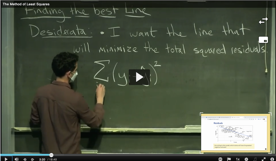
So how can we use this definition to decide precisely which intercept \(b_0\) and slopes \(b_1, b_2, \ldots, b_q\) to use? Please watch the following 19 minute video, “The Method of Least Squares”, to find out. The video is available in the media gallery on bcourses. Keep in mind that the video uses RSS instead of MSE. But RSS is just MSE multiplied by the sample size \(n\), so absolutely nothing changes.
Iterative Numerical Methods
As we saw in the video, the problem of least squares can be defined as one of optimization.
def: Ordinary Least Squares
Find the \(b_0,\ldots, b_q\) that make the following quantity \[\widehat{\mbox{MSE}} (b_0,b_1, \ldots, b_q) = \frac1{n} \sum_{i = 1}^n \left[Y_i - \left(b_{0} + b_1 X_{1,i} + \ldots +b_q X_{q,i} \right)\right]^2\]
the smallest possible.
The learned optimal solutions will be indicated by
\[\hat{b}_{0,OLS},\hat{b}_{1,OLS}, \ldots \hat{b}_{q,OLS} \]
so that finally \[\hat{Y}_{OLS}(\mathbf{X}) \equiv \hat{b}_{0,OLS} + \hat{b}_{1,OLS} X_1 + \hat{b}_{2,OLS} X_2 + \ldots +\hat{b}_{q,OLS} X_q \]
Although a direct way to find these values involves taking the partial derivatives of the third equation with respect to each coefficient \(b_0\), \(b_1\), …, \(b_q\), setting the resulting equation equal to \(0\), and solving for the coefficient, you could think about using a different, perhaps more intuitive method.
Consider picking a starting value for each of \(b_0\) through \(b_q\), plugging these into the third equation, and seeing what comes out. Then, try to pick another set of numbers that makes the result of the \(MSE\) equation smaller. Provided that you have a concerted method to pick the next set of numbers, you can repeat this process over and over until you find the set of numbers which yields the smallest value for \(MSE\). This process can be described as an iterative numerical (as opposed to an exact, or analytical, or closed-form) method to find the values of the coefficients \(b_0\) through \(b_q\).
There are many iterative algorithms that accomplish the same task, some better than others. Two examples:
- Nelder-Mead: an older and more general (and generally not as reliable!) algorithm. This is the one we showed you in the video.
- Gradient Descent: the most-used algorithm currently. Used to fit deep learning models.
Summary
Prediction is the task of guessing the value of a target variable (\(Y\)) for an unseen observation using its values of other variables that are known, \(X_j\), the features, leveraging their hopefully strong association with the target. The nature of \(Y\) determines the nature of the task (and the method to solve it): regression concerns the prediction of numerical target variables, classification concerns the prediction of categorical target variables. One such regression model is the least squares linear model, which uses the line that minimizes the residual sum of squares. Finding the value of the coefficients is a task that can be solved directly using calculus (in simple settings like this one) and also with optimization algorithms (in more general settings). We gave an example of using such an algorithm, demonstrating how to write a function in R in the process.
The fundamental difference between generalization and prediction
In both cases we are using old data to make guesses about new data.
However:
In generalization, we are guessing unknown and unobservable quantities (distribution/population parameters). You will never be able to check directly how close you got to the true \(\mu\), \(p\), \(\sigma\), etc…
In prediction, we are guessing presently unknown, but, in the future, in principle observable and knowable quantities (random variables). For example, you can ask the person if they are Guelph or a Ghibelline (good luck with that!).
This difference has massive consequences and that’s why Statistical Inference (i.e. generalization) and Machine Learning (i.e. prediction) are, in practice, regarded as two completely separate subjects.