| name | sleep_total | log_bodywt_g | vore | conservation |
|---|---|---|---|---|
| Cheetah | 12.1 | 10.8 | carni | lc |
| Owl monkey | 17.0 | 6.2 | omni | NA |
| Mountain beaver | 14.4 | 7.2 | herbi | nt |
| Greater short-tailed shrew | 14.9 | 2.9 | omni | lc |
| Cow | 4.0 | 13.3 | herbi | domesticated |
| Three-toed sloth | 14.4 | 8.3 | herbi | NA |
| Northern fur seal | 8.7 | 9.9 | carni | vu |
| Vesper mouse | 7.0 | 3.8 | NA | NA |
| Dog | 10.1 | 9.5 | carni | domesticated |
| Roe deer | 3.0 | 9.6 | herbi | lc |
Data Wrangling
Whipping your data into shape
WarningThis page covers…
- Data Wrangling
- Introduction to functions from the
dplyrpackage (part oftidyverse)filtermutateselectgroup_bysummarize
- Comparison operators:
==,!=,>,<,>=,<=
- The pipe
|>operator
Datasets aren’t always ready to make the plot you need. For many reasons.
Sometimes they need fixing or adjusting before you can even start. A measurement is in inches but you need it in centimeters. Some rows were duplicated by accident. There’s a bunch of columns you don’t need because they aren’t relevant to this task and are cluttering your screen. These “data cleaning” tasks are a major step in your work. Not just when data is dirty or broken, but when it’s not yet what you need.
Even then, you often still need to transform again to make some particular plot or table. Maybe you want to make a scatterplot, but only of Adelie penguins. Maybe you have some data on student quiz scores over a semester, and you want to only see everyone’s highest and lowest scores, not all the scores. These things aren’t straightforward to do with our tools so far.
The dplyr package, which comes along with tidyverse, offers many reshaping tools to serve this purpose. We’ll talk about its core functions (like filter and mutate), but also how to tell them what you want (using things like “comparison operators”). Along the way, we’ll begin using a new, very important piece of syntax: the pipe operator |>.
This is data wrangling.
Sleeping like a baby (orangutan)
How much do different kinds of animals sleep? Why? Today’s dataset, msleep, has some very interesting answers.
Researchers Van Savage and Geoffrey West studied the fitness value of sleep, in particular why some mammals seem to need more or less of it. They were especially interested in body size and metabolic rate (roughly how active vs lazy they are). They measured a truly wide range of mammals and published their data, which we’ll consider today.
Take a look at the first few rows of their data below. It’s in a dataframe already available to you: msleep (mammalian sleep).1
Each row is a species of mammal (so this is our “unit of observation”).
Each column is a specific detail we “observe” about that species:
namesleep_total: its average length of sleep each day, in hourslog_bodywt_g: the (natural log of) the species’ average body weight, in gramsvore: its dietary pattern (herbivore, etc)conservation: its conservation status (endangered, etc)
NoteFYI: the data has been altered from the raw
msleep to make the notes easier to follow. Click to see how.
In msleep, the only “weight” column is bodywt, which is in kilograms. It’s easier to work in grams (and log grams), so we make new columns for convenience: bodywt_g and log_bodywt_g. You will learn to understand this code by the end of these notes
msleep = msleep |>
    mutate(bodywt_g = bodywt * 1000,
           log_bodywt_g = log(bodywt_g) |> round(1))
We can visualize the relationship between “sleep amount” and “body weight” in all 83 species using a scatter plot.
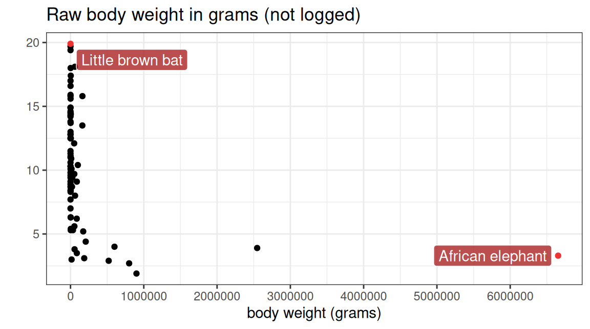
The mammals vary from the wee (10-gram) brown bat, slumbering for nearly 20 hours a day, to the massive (7,000-kilogram) African elephant, nodding off for less than five. That is quite a range! Let’s drill down to smaller subsets of this data frame to gain a more nuanced sense of what is going on.
NoteWhy do we use the log of body weight? (Optional)
Below is the regular, un-logged plot of body weight and sleep duration:
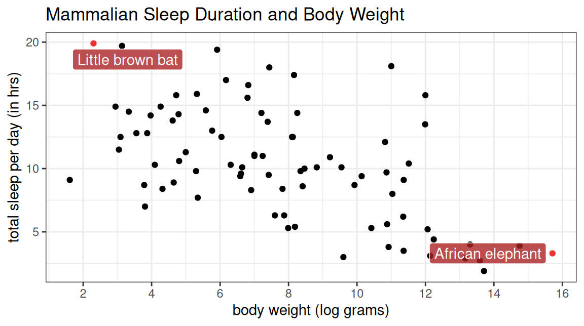
See a problem?
Mammals are a diverse bunch. They have an enormous range of body sizes; tiny shrews weighing 5 grams, and elephants weighing 7,000,000 grams. Most mammals are quite small, much closer to the 5-gram end of our range, so we end up with a useless plot that has mostly dots stacked up the y-axis.
In the plot above, mammal body sizes appear to be wildly asymmetrically distributed (strong right-skew). But it’s actually a pretty even distribution by order of magnitude. Roughly \(10^1\) to \(10^7\) (six orders apart, in base 10). Sleep durations don’t have this feature. They are roughly evenly distributed in the 2-20 range. As a result, the sleep durations fit just fine on a standard plot (they’re nicely spread out on the y-axis), but body weights do not (all the points look glued to the left side of the plot).
Taking the log fixes this problem. At their core, logarithms answer the very question, “what order of magnitude is this number?”
- After \(log_{10}\), the numbers 1, 10, 100, and 1000 become their magnitudes: 0, 1, 2, and 3.
- After \(log_e\), the numbers 1, \(e\), \(e^2\), and \(e^3\) become their magnitudes: 0, 1, 2, and 3.
Once you log the body weights, you see that they’re pretty evenly spread out across those orders of magnitude. On the logged plot, 10 and 100 grams (\(10^1\) and \(10^2\)) look exactly as far apart as 100 and 1000 grams (\(10^2\) and \(10^3\)). And there are similar numbers of mammals in those bands. With this transformation, we can comfortably see 10-gram, 1000-gram, and 1-million-gram animals all on the same plot. Look at the natural log plot again:
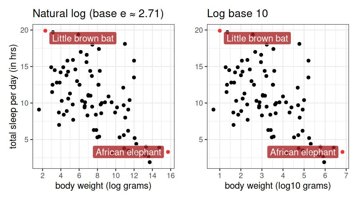
Math note: It doesn’t actually matter here if you take the natural log, the log base 10, or the log base 2. It still fixes the scaling problem: the x-axis numbers will just change. The plots below will demonstrate. The left plot is the same as the natural log plot above (log() in R). The second uses the log base 10 of body weight (log10() in R). There is only one difference in the resulting plots: the numbers on the x-axis are all about twice as big on the left. Because you have to raise \(e\) to roughly the 2nd power to get to 10.
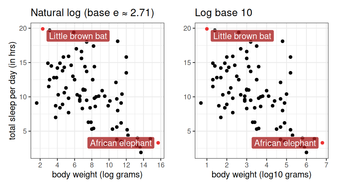
By convention, scientists use log base \(e\) in most situations. There are good reasons for this, but the downside is that the x-axis labels become hard to interpret. The ‘5’ on the left plot’s x-axis means \(e^5\), but nobody can easily calculate what actual number that is. As a result, in this course, you probably should use log10() when you are given a choice. Everything is just easier to interpret. A ‘5’ on the right plot’s x-axis means \(10^5\) which is 100,000. Easy enough. But you should be aware that natural log is generally the implied logarithm when a base isn’t specified, across most sciences.
Filtering - removing rows
In the plots above, it sort of looks like bigger animals sleep less, though it’s a blurry relationship. What else might be happening?
One way to start exploring is to “drill down” on a subset of the data. Maybe just carnivores. Maybe just small animals. Maybe just endangered species.
The filter function is our tool to extract a subset of rows from a dataset. filter is a function that takes at least two arguments: a dataset, and a condition that has to be met for the row to be kept. For example, to get all the carnivores, we could do:
filter(msleep, vore == "carni")| name | sleep_total | log_bodywt_g | vore | conservation |
|---|---|---|---|---|
| Cheetah | 12.1 | 10.8 | carni | lc |
| Northern fur seal | 8.7 | 9.9 | carni | vu |
| Dog | 10.1 | 9.5 | carni | domesticated |
| Long-nosed armadillo | 17.4 | 8.2 | carni | lc |
| Domestic cat | 12.5 | 8.1 | carni | domesticated |
| Pilot whale | 2.7 | 13.6 | carni | cd |
| Gray seal | 6.2 | 11.4 | carni | lc |
| Thick-tailed opposum | 19.4 | 5.9 | carni | lc |
| Slow loris | 11.0 | 7.2 | carni | NA |
| Northern grasshopper mouse | 14.5 | 3.3 | carni | lc |
All carnivores. Don’t worry about the specific syntax yet, we’ll talk more about it shortly.
An important note: this code does not change the original msleep dataframe. This confuses new programmers regularly. Instead, this code creates a completely new dataframe, one with only carnivores.
Let’s peek back at msleep to confirm that it is unchanged:
msleep| name | sleep_total | log_bodywt_g | vore | conservation |
|---|---|---|---|---|
| Cheetah | 12.1 | 10.8 | carni | lc |
| Owl monkey | 17.0 | 6.2 | omni | NA |
| Mountain beaver | 14.4 | 7.2 | herbi | nt |
| Greater short-tailed shrew | 14.9 | 2.9 | omni | lc |
| Cow | 4.0 | 13.3 | herbi | domesticated |
| Three-toed sloth | 14.4 | 8.3 | herbi | NA |
| Northern fur seal | 8.7 | 9.9 | carni | vu |
| Vesper mouse | 7.0 | 3.8 | NA | NA |
| Dog | 10.1 | 9.5 | carni | domesticated |
| Roe deer | 3.0 | 9.6 | herbi | lc |
All ’vores are accounted for. Now let’s plot just the carnivores to see if a pattern is clearer:
ggplot(filter(msleep, vore == "carni"),
       aes(x = log_bodywt_g, y = sleep_total)) +
    geom_point() +
    labs(title = "Carnivore body weight (log scale) vs sleep duration")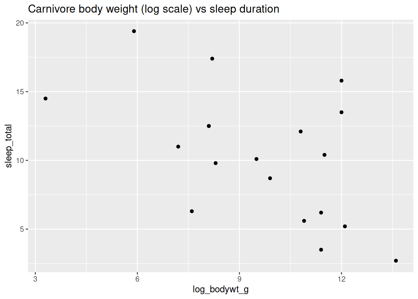
Comparison Operators
Notice anything funny in the code we just used?
filter(msleep, vore == "carni")The code above uses two equals signs together: vore == "carni". Why not just one equals, vore = "carni"?
Important detail: single = vs double ==
Single = and double == do fundamentally different things in R (and most coding languages):
- A single
=is a command. It says “make these things equal.”- Variable assignment:
x = 4says “MAKE x equal to 4.” We are setting a variablexto the value 4. (Though we usually do variable assignment with an arrow,x <- 4, it’s also valid to dox = 4). - Named arguments to functions: when we write
mean(numbers, na.rm = TRUE), thena.rm = TRUEpart says “MAKE the na.rm argument equal to TRUE” (recall: this is how we remove missing values (NAs) from a vector before trying to average them).
- Variable assignment:
- A double
==is a question. It asks, “are these things equal?” The answer is yes or no (TRUE or FALSE).x == 2asks “IS x equal to 2?” The answer will be TRUE or FALSE depending on x’s value.- If you have a vector, using
==will ask the question of every element in the vector and return a vector of TRUEs and FALSEs.
Some simple examples demonstrating = and ==
x = 4With a single =, this line makes x equal to 4. There is no output printed, as we are simply assigning a variable a value.
x == 4[1] TRUEWith the double ==, this line asks if x is equal to 4. Since we just set x to be 4, the output on your screen says TRUE.
numbers = c(1, 2, 3)
numbers == 2
[1] FALSE TRUE FALSEThe first line with the single = says “MAKE the numbers variable equal to the vector (1, 2, 3).” (Again, this is equivalent to numbers <- c(1, 2, 3)). The second line with the double == asks, for each element in the vector, “is this number equal to 2?” The output is a logical vector of the answers: FALSE TRUE FALSE. Only the second number in numbers is equal to 2.
So earlier, when we ran:
filter(msleep, vore == "carni")R went through every row and noted where the condition was true (vore was equal to “carni”). It then gave us a new dataframe with only these rows.
More comparison operators
The double == is one of many ways to ask a question about two things. In this case, == asks “are they equal?”. But this is only one of many ways to compare two things. There are many more such “comparison operators”:
| Operator | Translation | Example |
|---|---|---|
== |
equal to? | 4 == 6 returns FALSE |
!= |
not equal to? | 4 != 6 returns TRUE |
< |
less than? | 4 < 6 returns TRUE, while 4 < 4 returns FALSE |
<= |
less than or equal to? | 4 <= 6 returns TRUE, and 4 <= 4 also returns TRUE |
> |
greater than? | 4 > 6 returns FALSE |
>= |
greater than or equal to? | 4 >= 6 returns FALSE |
%in% |
asks if the thing on the left is IN the vector on the right | 3 %in% c(1, 3, 5) returns TRUE |
Let’s try some of these out. Let’s filter for only the rows with large animals, defined as those with a log body weight greater than 12.
filter(msleep, log_bodywt_g > 12)| name | sleep_total | log_bodywt_g | vore | conservation |
|---|---|---|---|---|
| Cow | 4.0 | 13.3 | herbi | domesticated |
| Asian elephant | 3.9 | 14.8 | herbi | en |
| Horse | 2.9 | 13.2 | herbi | domesticated |
| Donkey | 3.1 | 12.1 | herbi | domesticated |
| Giraffe | 1.9 | 13.7 | herbi | cd |
| Pilot whale | 2.7 | 13.6 | carni | cd |
| African elephant | 3.3 | 15.7 | herbi | vu |
| Brazilian tapir | 4.4 | 12.2 | herbi | vu |
| Bottle-nosed dolphin | 5.2 | 12.1 | carni | NA |
There were 9 such animals. Reading the names confirms that, yes, these are the big ones.
Multiple criteria? Use logical operators to join them.
What if you want to extract only the creatures that are both very large and short-sleeping ? Well, for that, we need to do more than one comparison. We stitch these comparisons together with “logical operators”: & (“and”), | (“or”).
This filter returns the creatures who are large AND sleep little.
filter(msleep, log_bodywt_g > 12 & sleep_total < 5)| name | sleep_total | log_bodywt_g | vore | conservation |
|---|---|---|---|---|
| Cow | 4.0 | 13.3 | herbi | domesticated |
| Asian elephant | 3.9 | 14.8 | herbi | en |
| Horse | 2.9 | 13.2 | herbi | domesticated |
| Donkey | 3.1 | 12.1 | herbi | domesticated |
| Giraffe | 1.9 | 13.7 | herbi | cd |
| Pilot whale | 2.7 | 13.6 | carni | cd |
| African elephant | 3.3 | 15.7 | herbi | vu |
| Brazilian tapir | 4.4 | 12.2 | herbi | vu |
This can be read as “make me a dataframe with the rows from msleep where the log body weight is greater than 12 and the sleep total is less than 5.” We see that there are 8 such creatures, one fewer than the data frame with only the body weight filter. The bottle-nosed dolphin is a relatively big mammal thatsleeps, on average, 5.2 hrs.
This next block of code returns the creatures who are large OR sleep little. All we have to do is change & (and) to | (or).
filter(msleep, log_bodywt_g > 12 | sleep_total < 5)| name | sleep_total | log_bodywt_g | vore | conservation |
|---|---|---|---|---|
| Cow | 4.0 | 13.3 | herbi | domesticated |
| Roe deer | 3.0 | 9.6 | herbi | lc |
| Asian elephant | 3.9 | 14.8 | herbi | en |
| Horse | 2.9 | 13.2 | herbi | domesticated |
| Donkey | 3.1 | 12.1 | herbi | domesticated |
| Giraffe | 1.9 | 13.7 | herbi | cd |
| Pilot whale | 2.7 | 13.6 | carni | cd |
| African elephant | 3.3 | 15.7 | herbi | vu |
| Sheep | 3.8 | 10.9 | herbi | domesticated |
| Caspian seal | 3.5 | 11.4 | carni | vu |
| Brazilian tapir | 4.4 | 12.2 | herbi | vu |
| Bottle-nosed dolphin | 5.2 | 12.1 | carni | NA |
This filter is much more permissive - we keep all the big ones (no matter how long they sleep) and all the short-sleeping ones (no matter their size).
This permits animals like the Roe deer, which is not a particularly large mammal (log body weight of only 9.6) but who sleeps only 3 hours a day. We also get the Bottle-nosed dolphin, who is not a short sleeper (5.2 hours/day) but is large (log body weight of 12.1).
These conditional expressions can get arbitrarily complex, using parentheses to group things. Try to intuit what the following code does:
filter(msleep, vore == "herbi" & (sleep_total < 5 | sleep_total > 15))| name | sleep_total | log_bodywt_g | vore | conservation |
|---|---|---|---|---|
| Cow | 4.0 | 13.3 | herbi | domesticated |
| Roe deer | 3.0 | 9.6 | herbi | lc |
| Asian elephant | 3.9 | 14.8 | herbi | en |
| Horse | 2.9 | 13.2 | herbi | domesticated |
| Donkey | 3.1 | 12.1 | herbi | domesticated |
| Giraffe | 1.9 | 13.7 | herbi | cd |
| African elephant | 3.3 | 15.7 | herbi | vu |
| Sheep | 3.8 | 10.9 | herbi | domesticated |
| Arctic ground squirrel | 16.6 | 6.8 | herbi | lc |
| Golden-mantled ground squirrel | 15.9 | 5.3 | herbi | lc |
| Eastern american chipmunk | 15.8 | 4.7 | herbi | NA |
| Brazilian tapir | 4.4 | 12.2 | herbi | vu |
This looks for rows where the animal is an herbivore (vore == "herbi") and it either sleeps very little or a whole lot ((sleep_total < 5 | sleep_total > 15)). There are 12 such animals, including fun ones like the “Golden-mantled ground squirrel” (a long-sleeping herbivore) and the giraffe (a short-sleeping herbivore).
When working with nominal categorical variables, the only operators that you’ll be using are == and !=. You can return a union like normal using |,
filter(msleep, name == "Little brown bat" | name == "African elephant")| name | genus | vore | order | conservation | sleep_total | sleep_rem | sleep_cycle | awake | brainwt | bodywt | bodywt_g | log_bodywt_g |
|---|---|---|---|---|---|---|---|---|---|---|---|---|
| African elephant | Loxodonta | herbi | Proboscidea | vu | 3.3 | NA | NA | 20.7 | 5.71200 | 6654.00 | 6654000 | 15.7 |
| Little brown bat | Myotis | insecti | Chiroptera | NA | 19.9 | 2 | 0.2 | 4.1 | 0.00025 | 0.01 | 10 | 2.3 |
Translation: Only the brown bat and African elephant.
filter(msleep, name != "Little brown bat" & name != "African elephant")| name | sleep_total | log_bodywt_g | vore | conservation |
|---|---|---|---|---|
| Cheetah | 12.1 | 10.8 | carni | lc |
| Owl monkey | 17.0 | 6.2 | omni | NA |
| Mountain beaver | 14.4 | 7.2 | herbi | nt |
| Greater short-tailed shrew | 14.9 | 2.9 | omni | lc |
| Cow | 4.0 | 13.3 | herbi | domesticated |
| Three-toed sloth | 14.4 | 8.3 | herbi | NA |
| Northern fur seal | 8.7 | 9.9 | carni | vu |
| Vesper mouse | 7.0 | 3.8 | NA | NA |
| Dog | 10.1 | 9.5 | carni | domesticated |
| Roe deer | 3.0 | 9.6 | herbi | lc |
Translation: Everything but the brown bat and the elephant.
Or you can save some typing (and craft more readable code) by using %in% instead, followed by a vector of possible matches:
filter(msleep, name %in% c("Little brown bat", "African elephant"))# A tibble: 2 × 13
name genus vore order conservation sleep_total sleep_rem sleep_cycle awake
<chr> <chr> <chr> <chr> <chr> <dbl> <dbl> <dbl> <dbl>
1 Africa… Loxo… herbi Prob… vu 3.3 NA NA 20.7
2 Little… Myot… inse… Chir… <NA> 19.9 2 0.2 4.1
# ℹ 4 more variables: brainwt <dbl>, bodywt <dbl>, bodywt_g <dbl>,
# log_bodywt_g <dbl>select - removing columns
select gets rid of columns. It creates a new dataframe with only the columns you specify, in the order you specify them.
This is common with real world datasets, which often have a lot more information than you need for your particular analysis. Removing unnecessary columns makes your screen less cluttered and your code clearer.
Let’s pare down the msleep dataset to just three columns: name, log_bodywt_g, and sleep_total. You can see that the select function takes a dataset as its first argument, then any number of column names as subsequent arguments:
select(msleep, name, log_bodywt_g, sleep_total)| name | log_bodywt_g | sleep_total |
|---|---|---|
| Cheetah | 10.8 | 12.1 |
| Owl monkey | 6.2 | 17.0 |
| Mountain beaver | 7.2 | 14.4 |
| Greater short-tailed shrew | 2.9 | 14.9 |
| Cow | 13.3 | 4.0 |
| Three-toed sloth | 8.3 | 14.4 |
| Northern fur seal | 9.9 | 8.7 |
| Vesper mouse | 3.8 | 7.0 |
| Dog | 9.5 | 10.1 |
| Roe deer | 9.6 | 3.0 |
The code above says, “Please give me a new dataset with only the name, log_bodywt_g, and sleep_total columns from msleep”.
Again, this does not change the original msleep dataframe. It makes a new one. If you wanted to replace msleep with this new, smaller dataset, you would have to assign it back to msleep:
msleep <- select(msleep, name, log_bodywt, sleep_total)This is common. You load a new, complex dataset. You get rid of things you don’t need, overwriting the original dataframe with the reduced version. Don’t be afraid to do this in your work. (But if you end up mangling your dataframe by accident, you can restart R and reset yourself.)
Inverse selection - specify what to drop, not what to keep
You can also use - to say “Everything but this column.” For example, to get a copy of msleep with everything but the conservation and vore columns, you could do:
select(msleep, -conservation, -vore)| name | sleep_total | log_bodywt_g |
|---|---|---|
| Cheetah | 12.1 | 10.8 |
| Owl monkey | 17.0 | 6.2 |
| Mountain beaver | 14.4 | 7.2 |
| Greater short-tailed shrew | 14.9 | 2.9 |
| Cow | 4.0 | 13.3 |
| Three-toed sloth | 14.4 | 8.3 |
| Northern fur seal | 8.7 | 9.9 |
| Vesper mouse | 7.0 | 3.8 |
| Dog | 10.1 | 9.5 |
| Roe deer | 3.0 | 9.6 |
NoteA trick to remembering
select vs filter
filter and row have an r in them, while select and column both have a c. So filter is for rows, select is for columns.
mutate - modifying or adding columns
To add a new column, or to alter an existing column, we use mutate.
mutate is a function. It takes two arguments: a dataframe, and instructions on what column to make or change.
For example, let’s add a new column to our msleep dataset, sleep_total_minutes, which is the animal’s total sleep per day in minutes instead of hours:
mutate(msleep, sleep_total_minutes = sleep_total * 60)| name | sleep_total | log_bodywt_g | vore | conservation | sleep_total_minutes |
|---|---|---|---|---|---|
| Cheetah | 12.1 | 10.8 | carni | lc | 726 |
| Owl monkey | 17.0 | 6.2 | omni | NA | 1020 |
| Mountain beaver | 14.4 | 7.2 | herbi | nt | 864 |
| Greater short-tailed shrew | 14.9 | 2.9 | omni | lc | 894 |
| Cow | 4.0 | 13.3 | herbi | domesticated | 240 |
| Three-toed sloth | 14.4 | 8.3 | herbi | NA | 864 |
| Northern fur seal | 8.7 | 9.9 | carni | vu | 522 |
| Vesper mouse | 7.0 | 3.8 | NA | NA | 420 |
| Dog | 10.1 | 9.5 | carni | domesticated | 606 |
| Roe deer | 3.0 | 9.6 | herbi | lc | 180 |
Instead of making a whole new column, you could change the meaning of the existing sleep_total to just be in minutes. You can modify a column in-place like so:
mutate(msleep, sleep_total = sleep_total * 60)| name | sleep_total | log_bodywt_g | vore | conservation |
|---|---|---|---|---|
| Cheetah | 726 | 10.8 | carni | lc |
| Owl monkey | 1020 | 6.2 | omni | NA |
| Mountain beaver | 864 | 7.2 | herbi | nt |
| Greater short-tailed shrew | 894 | 2.9 | omni | lc |
| Cow | 240 | 13.3 | herbi | domesticated |
| Three-toed sloth | 864 | 8.3 | herbi | NA |
| Northern fur seal | 522 | 9.9 | carni | vu |
| Vesper mouse | 420 | 3.8 | NA | NA |
| Dog | 606 | 9.5 | carni | domesticated |
| Roe deer | 180 | 9.6 | herbi | lc |
Again, none of this has changed msleep! Each line above made a whole new dataframe. If we wanted to change our msleep dataset itself, we would have to assign this new dataframe back to msleep:
msleep <- mutate(msleep, sleep_total = sleep_total * 60)Code like this is common practice. At the start of your analysis, make the columns mean what you need them to mean, remove what you don’t need, then get to work. For example, if you know you want to work in “minutes” of sleep in your research, just change the column in place, as above.
arrange - sorting your rows
arrange sorts your dataframe rows according to a column you specify. Like the others, arrange generates a new dataframe, it doesn’t modify your old one unless you explicitly set it to do so (as above).
arrange is a function expecting two arguments: the dataset, and the column to sort on.
To sort by name (A-Z):
arrange(msleep, name)| name | sleep_total | log_bodywt_g | vore | conservation |
|---|---|---|---|---|
| African elephant | 3.3 | 15.7 | herbi | vu |
| African giant pouched rat | 8.3 | 6.9 | omni | NA |
| African striped mouse | 8.7 | 3.8 | omni | NA |
| Arctic fox | 12.5 | 8.1 | carni | NA |
| Arctic ground squirrel | 16.6 | 6.8 | herbi | lc |
| Asian elephant | 3.9 | 14.8 | herbi | en |
| Baboon | 9.4 | 10.1 | omni | NA |
| Big brown bat | 19.7 | 3.1 | insecti | lc |
| Bottle-nosed dolphin | 5.2 | 12.1 | carni | NA |
| Brazilian tapir | 4.4 | 12.2 | herbi | vu |
To sort by sleep duration (low to high):
arrange(msleep, sleep_total)| name | sleep_total | log_bodywt_g | vore | conservation |
|---|---|---|---|---|
| Giraffe | 1.9 | 13.7 | herbi | cd |
| Pilot whale | 2.7 | 13.6 | carni | cd |
| Horse | 2.9 | 13.2 | herbi | domesticated |
| Roe deer | 3.0 | 9.6 | herbi | lc |
| Donkey | 3.1 | 12.1 | herbi | domesticated |
| African elephant | 3.3 | 15.7 | herbi | vu |
| Caspian seal | 3.5 | 11.4 | carni | vu |
| Sheep | 3.8 | 10.9 | herbi | domesticated |
| Asian elephant | 3.9 | 14.8 | herbi | en |
| Cow | 4.0 | 13.3 | herbi | domesticated |
To sort by a column from high to low, we need to wrap our column name in a function, desc() (for “descending”)
arrange(msleep, desc(sleep_total))| name | sleep_total | log_bodywt_g | vore | conservation |
|---|---|---|---|---|
| Little brown bat | 19.9 | 2.3 | insecti | NA |
| Big brown bat | 19.7 | 3.1 | insecti | lc |
| Thick-tailed opposum | 19.4 | 5.9 | carni | lc |
| Giant armadillo | 18.1 | 11.0 | insecti | en |
| North American Opossum | 18.0 | 7.4 | omni | lc |
| Long-nosed armadillo | 17.4 | 8.2 | carni | lc |
| Owl monkey | 17.0 | 6.2 | omni | NA |
| Arctic ground squirrel | 16.6 | 6.8 | herbi | lc |
| Golden-mantled ground squirrel | 15.9 | 5.3 | herbi | lc |
| Tiger | 15.8 | 12.0 | carni | en |
arrange is useful when you are trying to present data (to yourself or others) in a natural order. It’s also useful if you’re trying to find the largest or smallest value (e.g. the shortest-sleeping animal, which is the Giraffe in this dataset).
group_by - different calculations for different groups
group_by is inherently a helper function. It takes two arguments: a dataframe, and a column to use to define “groups.” It returns a copy of the same full dataframe with only one change: it has quietly made note of which rows belong to which groups. For example, if we group msleep by vore (dietary habits), it will make note of which rows are carnivores, which are omnivores, etc.
Why bother? group_by does nothing useful on its own, but many downstream functions like summarize use these groups to change how they behave.
First, notice that group_by returns the whole dataframe, unchanged, but with a special “groups” note:
Original dataset (not grouped)
msleep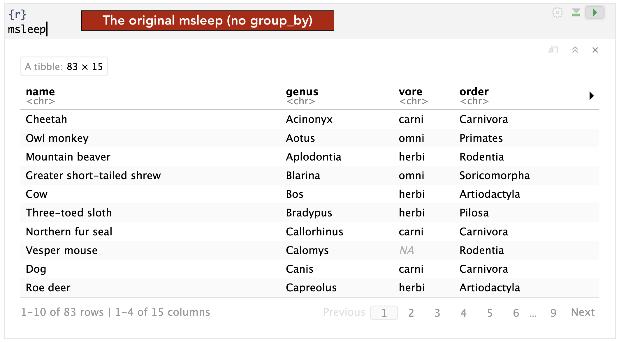
After group_by
group_by(msleep, vore)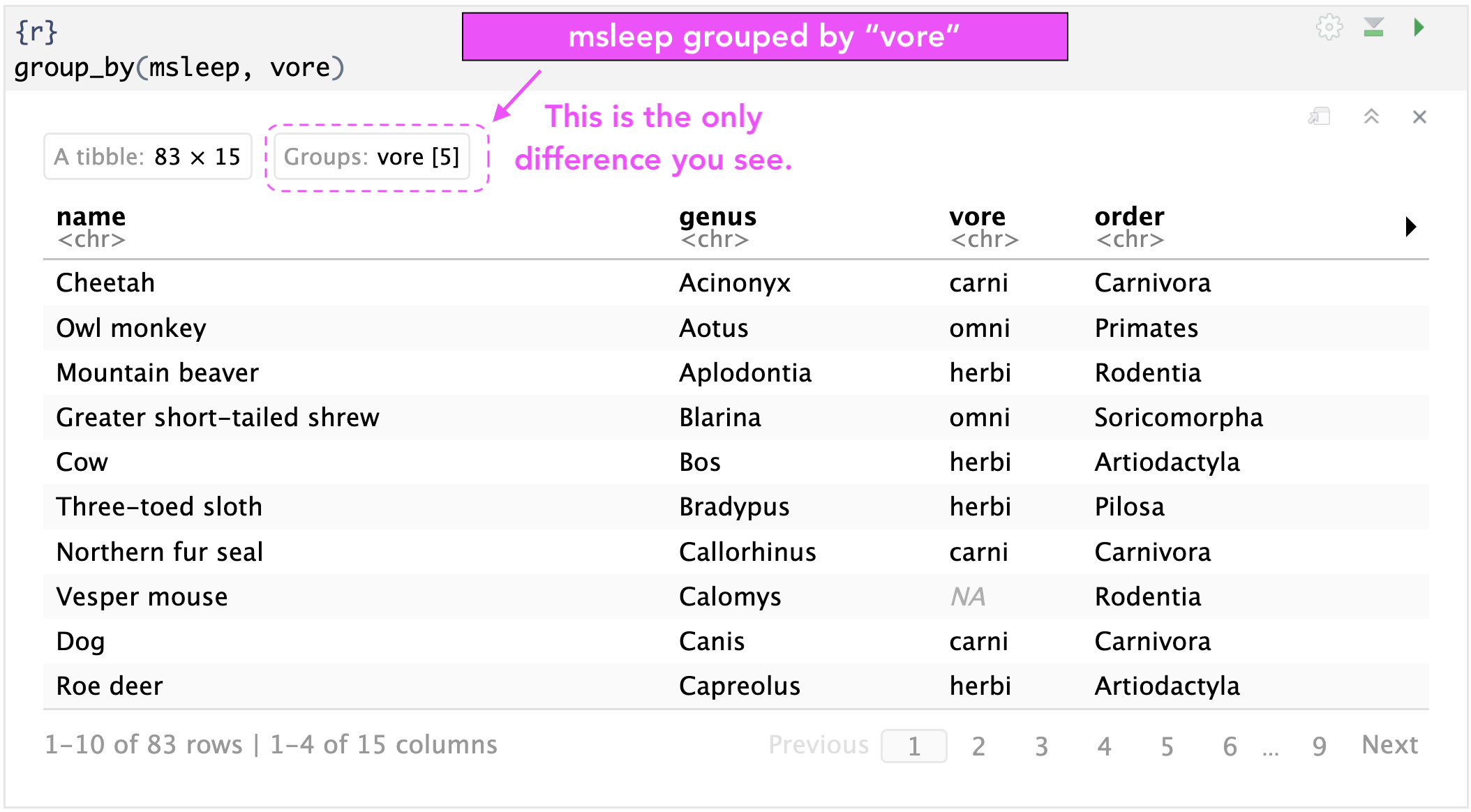
There’s actually a lot more you can do with group_by – e.g., find the longest-sleeping animal of each vore type – but this is beyond our scope for now.
How summarize changes when given grouped data
Without grouping:
summarize(msleep, mean_sleep_duration = mean(sleep_total, na.rm = TRUE))| mean_sleep_duration |
|---|
| 10.43373 |
This is just the mean sleep duration across all mammals. However, if we group by vore first…
summarize(group_by(msleep, vore), mean_sleep_duration = mean(sleep_total, na.rm = TRUE))| vore | mean_sleep_duration |
|---|---|
| carni | 10.378947 |
| herbi | 9.509375 |
| insecti | 14.940000 |
| omni | 10.925000 |
| NA | 10.185714 |
…we get the calculation once for each group.
The Almighty “Pipe”
It is SO common to do many data wrangling steps at once. It’s typical that, after you get some data, you need to do some filtering, mutating, etc before you are ready to do your analysis or make your plot.
The problem? When you chain together a bunch of functions in R, it can get messy. Consider:
sqrt(mean(c(1, 2, 3)))You have to stare at this for a minute to see what it’s doing. As we discussed, nested functions like this (c within mean within sqrt) are evaluated from the inside out. In diagram form, this is what’s happening:
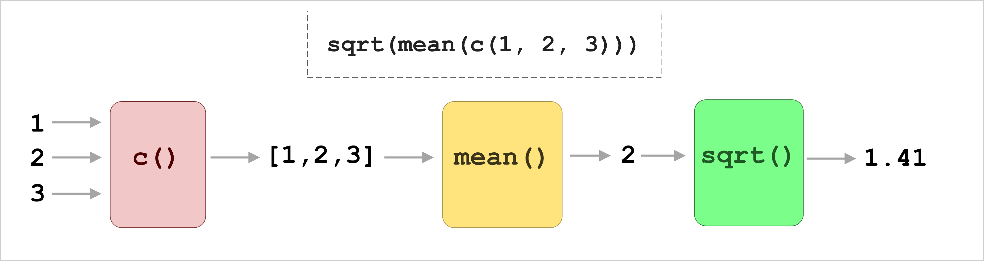
The diagram is a lot more intuitive. Data flows from left to right through a series of transformations. Wouldn’t it be nice if we could write our code more like this?
This is where the pipe operator |> comes in. (It’s composed of a vertical line (shift + backslash on most keyboards) followed by a greater than sign.)
Before we explain further, here’s the punchline: using the pipe, you can rewrite the line of code above as c(1, 2, 3) |> mean() |> sqrt().
First, notice how naturally this reads. We make a vector with some numbers, then compute their mean, then take the square root.
Especially in making plots or filtering/cleaning data, you often call a lot of functions in a row on the same dataset. First you filter out some rows, then you mutate to add a column, then maybe you do a group_by and summarize. Doing it all at once is a mess:
summarize(group_by(mutate(filter(msleep, log_bodywt > 12),
                          sleep_per_weight = sleep_total / log_bodywt),
                   vore),
          mean_sleep = mean(sleep_per_weight))
The pipe |> operator saves us. Literally all the pipe does is this: whatever is on the left side of the pipe is passed as the first argument to the function on the right side. The right side is always a function call.
With the pipe, we can rewrite sqrt(mean(c(1, 2, 3))) as c(1, 2, 3) |> mean() |> sqrt(). This code is functionally exactly the same.
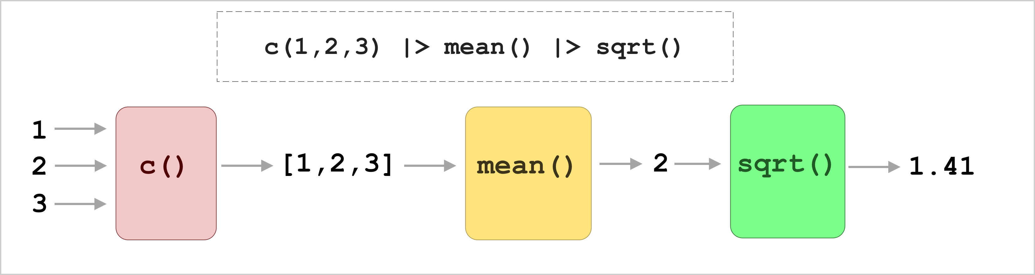
Let’s walk through the code itself, left to right. First, we see c(1, 2, 3) |> mean(). The stuff to the left of the pipe, c(1, 2, 3), is moved into the function on the right (mean). The result is that it runs mean(c(1, 2, 3)).
Then there’s another pipe. So what’s now on the left, mean(c(1, 2, 3)), is moved into the function on the right, sqrt, to give us sqrt(mean(c(1, 2, 3))).
Here’s a quick animation to give you the idea if it’s still confusing:
Now let’s rewrite this gnarly code with pipes:
summarize(group_by(mutate(filter(msleep, log_bodywt > 12),
                          sleep_per_weight = sleep_total / log_bodywt),
                   vore),
          mean_sleep = mean(sleep_per_weight))
With pipes, it becomes:
msleep |>
    filter(log_bodywt > 12) |>
    mutate(sleep_per_weight = sleep_total / log_bodywt) |>
    group_by(vore) |>
    summarize(mean_sleep = mean(sleep_per_weight))
SO much better to read. Same result. We start with the msleep data frame, then filter some rows, then mutate to make a new column, then group by something, and finally summarize those groups. The data flows in a natural reading order through a series of transformations.
The code above is a very common kind of thing we do in data science. We alter a dataset through a series of steps, then end with a summary table or maybe a plot. The pipe, as you saw above, makes these things far more legible.
Let’s look at another example:
What proportion of carnivores sleep more than 8 hours daily?
Answering this requires two steps: filter()ing to focus on carnivores and summarize()ing to compute the proportion that meet a condition (recall that a comparison results in a logical vector of 0s and 1s). It is often a good idea to record the number of observations that go into a summary statistic, which we do here with the special summary function n().
msleep |>
    filter(vore == "carni") |>
    summarize(prop_over_8hrs = mean(sleep_total > 8),
              n = n())
# A tibble: 1 × 2
prop_over_8hrs n
<dbl> <int>
1 0.684 19What year had the greatest total number of christenings?
The original arbuthnot data frame, which captures birth records in 17th century London, in fact records the numbers of boys’ and girls’ names that appear in church christening records. To find the year with the greatest total number of christenings requires first the creation of a new column with mutate(), then arrange()ing the rows of that data frame, then (to not clutter our screen) select()ing just the columns of interest. As one pipeline, that is:
arbuthnot |>
    mutate(total = boys + girls) |>
    arrange(desc(total)) |>
    select(year, total)
# A tibble: 82 × 2
year total
<int> <int>
1 1705 16145
2 1707 16066
3 1698 16052
4 1708 15862
5 1697 15829
6 1702 15687
7 1701 15616
8 1703 15448
9 1706 15369
10 1699 15363
# ℹ 72 more rowsWhat is the trend in the total number of christenings over time?
arbuthnot |>
    mutate(total = boys + girls) |>
    ggplot(aes(x = year, y = total)) +
    geom_line()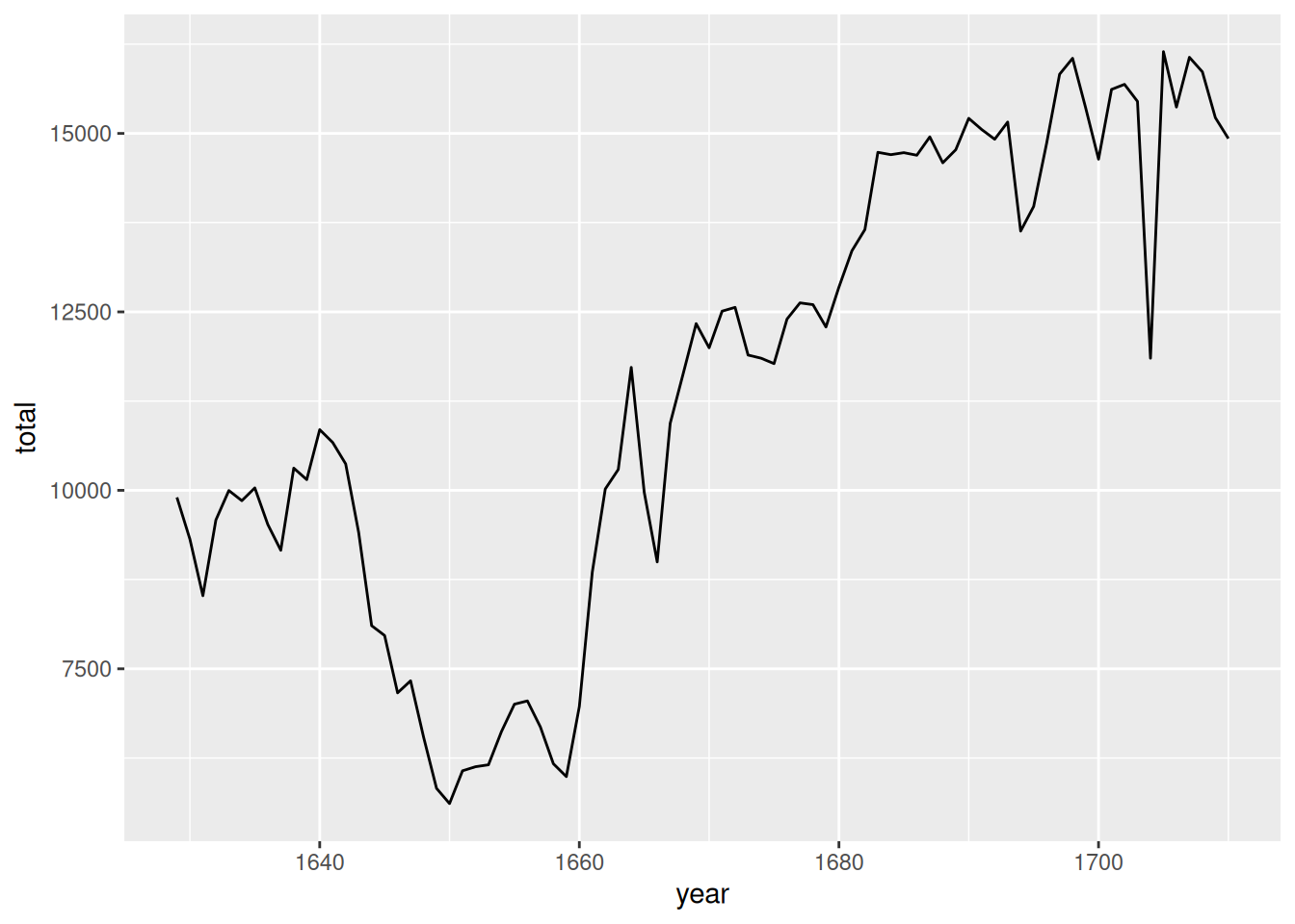
This demonstrates that you can pipe a data frame directly into a ggplot - the first argument is a data frame after all! The main thing to note is that when moving into a ggplot, the layers are added with the + operator instead of the pipe, |>.
Summary
The dplyr package, which comes along with tidyverse, offers some very useful tools for reshaping our data: arrange, filter, select, summarize, and group_by. The most important for data analysis is probably filtering: we often want to look at a subset of the rows that meet some condition (e.g., only animals over some body size, or only female penguins, etc.). We learned about comparison operators (==, <, etc.), joining multiple comparisons with the logical operators (& |), and how the pipe |> makes our code much easier to follow.
Footnotes
V. M. Savage and G. B. West. A quantitative, theoretical framework for understanding mammalian sleep. Proceedings of the National Academy of Sciences, 104 (3):1051-1056, 2007.↩︎